

Dissecting Zero #1: From Polynomials to Proofs, How Jolt Pro Proves Computation
A guide for engineers who want to understand what actually happens inside a zkVM.

Why this matters
All blockchains today operate in the same way. When a block is proposed, every validator re-executes every transaction to verify the result. If there are 100 validators, the same computation is repeated 100 times. This is how blockchains ensure correctness. “I ran it too, and got the same result, so it must be correct.”
It works, but it is fundamentally wasteful.
Succinct proofs, often grouped under the term “ZK,” propose a different approach. Instead of re-execution, an executor generates a mathematical proof that the computation was performed correctly. Validators verify only the proof. A computation that takes a billion steps to execute can be verified in roughly thirty.
First, clarify the terminology. “Zero-knowledge” strictly refers to a privacy property, where nothing is revealed beyond the validity of the proof. For blockchain scaling, the more important property is succinctness. Regardless of how large the original computation is, the proof remains small and verification remains fast. Jolt Pro currently implements succinct proofs. Full zero-knowledge privacy is on the near-term roadmap. In this article, “ZK” refers primarily to verifiable succinct computation, not privacy.
This is the core idea behind LayerZero’s Zero chain and its proving system, Jolt Pro. Most explanations of these systems either stay at an abstract "math magic" level or jump directly into research papers. This one starts from basic questions such as what polynomials are and why they are useful for detecting false claims, and builds up to how Jolt Pro proves 1.61 billion RISC-V cycles per second.
Finite fields: where the math happens
Before discussing proofs, we need to define the environment where the math operates.
Standard arithmetic uses an infinite sequence of numbers: 1, 2, 3, and so on. Computers cannot handle infinity, and cryptographic protocols require exact arithmetic without rounding errors. The solution is a finite field. It is a number system with a finite set of elements where addition, subtraction, multiplication, and division all work cleanly.
Think of a clock. On a 12-hour clock, 10 + 5 equals 3, not 15. Once it exceeds 12, it wraps around. A finite field follows the same idea, but uses a prime number p instead of 12.
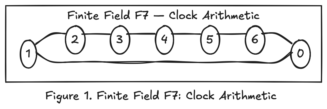
In the finite field F₇ = {0, 1, 2, 3, 4, 5, 6}, all operations are performed modulo 7:
Addition: 3 + 5 = 8 mod 7 = 1
Multiplication: 3 × 4 = 12 mod 7 = 5
Division: 3 / 2 = 3 × (inverse of 2) = 3 × 4 = 12 mod 7 = 5
Division works through multiplicative inverses. In F₇, the inverse of 2 is 4 because 2 × 4 = 8, and 8 mod 7 = 1. Every non-zero element has an inverse, which is why the modulus must be prime. If it is composite, some elements do not have inverses, and division breaks.
Why does ZK use finite fields? Two reasons. First, computers can perform exact integer arithmetic without floating point errors. Second, the security of ZK protocols depends on sampling random values from a large set. In practice, ZK systems use prime fields with around 2^256 elements. The space is large enough that randomly hitting a “bad” value is effectively impossible.
Polynomials: why lying fails
The central object is the polynomial.
A polynomial is a function composed of addition, multiplication, and exponentiation of variables:
f(x) = 3x² + 2x + 1
If x = 2, then f(2) = 12 + 4 + 1 = 17.
Polynomials have structural properties that are extremely useful for proofs.
A line is determined by two points.
Consider a degree-1 polynomial f(x) = ax + b. There are two unknowns, a and b. One point, for example f(1) = 5, is not enough. There are infinitely many lines passing through a single point. But two points, such as f(1) = 5 and f(3) = 11, produce two equations:
a + b = 5
3a + b = 11
Solving gives a = 3 and b = 2. There is exactly one line that passes through both points.
A parabola is determined by three points.
For a degree-2 polynomial f(x) = ax² + bx + c, there are three unknowns. Three points determine it uniquely.
General rule. A degree d polynomial has d + 1 unknowns, and is uniquely determined by d + 1 points. This implies:
Two different degree-d polynomials can agree on at most d points.
If they agree on more than d points, they must be the same polynomial.
Schwartz-Zippel lemma: catching lies with randomness
This property becomes a lie detector.
Suppose a prover claims a polynomial f(x), but the true polynomial is g(x), and f ≠ g. Both have degree at most d. Their difference h(x) = f(x) − g(x) is a non-zero polynomial of degree at most d. Therefore, h(x) = 0 for at most d values.
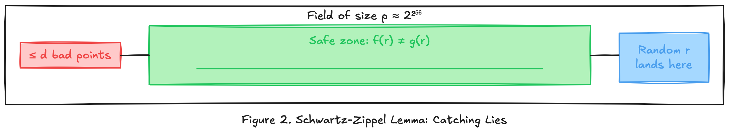
If a verifier picks a random point r from a finite field of size p:
Pr[f(r) = g(r)] ≤ d / p
If d = 1,000,000 and p = 2^256, the probability is about 10^-71.
This is the Schwartz-Zippel lemma. A single random evaluation detects a false polynomial with overwhelming probability. This fact underlies most ZK proof systems.
Sum-Check protocol: efficient verification
The Sum-Check protocol applies polynomial lie-detection to computation.
The problem
Given a multivariate polynomial f(x, y), we want to verify the sum over all binary inputs:
H = f(0,0) + f(0,1) + f(1,0) + f(1,1)
With m variables, there are 2^m terms. For m = 30, that is about one billion evaluations. The verifier cannot afford to compute this directly.
The prover claims H = 14. Can the verifier check this without computing all 2^m terms?
The core idea
The Sum-Check protocol reduces the problem one variable at a time.
Instead of checking the whole sum at once, the verifier asks the prover to “partially evaluate” the polynomial. In each round, one variable is replaced by a random challenge, and the remaining sum shrinks by half. After m rounds, the sum reduces to a single point evaluation, which the verifier can check directly.
At each step, the Schwartz-Zippel lemma guarantees that a dishonest prover is caught with overwhelming probability.
Walkthrough
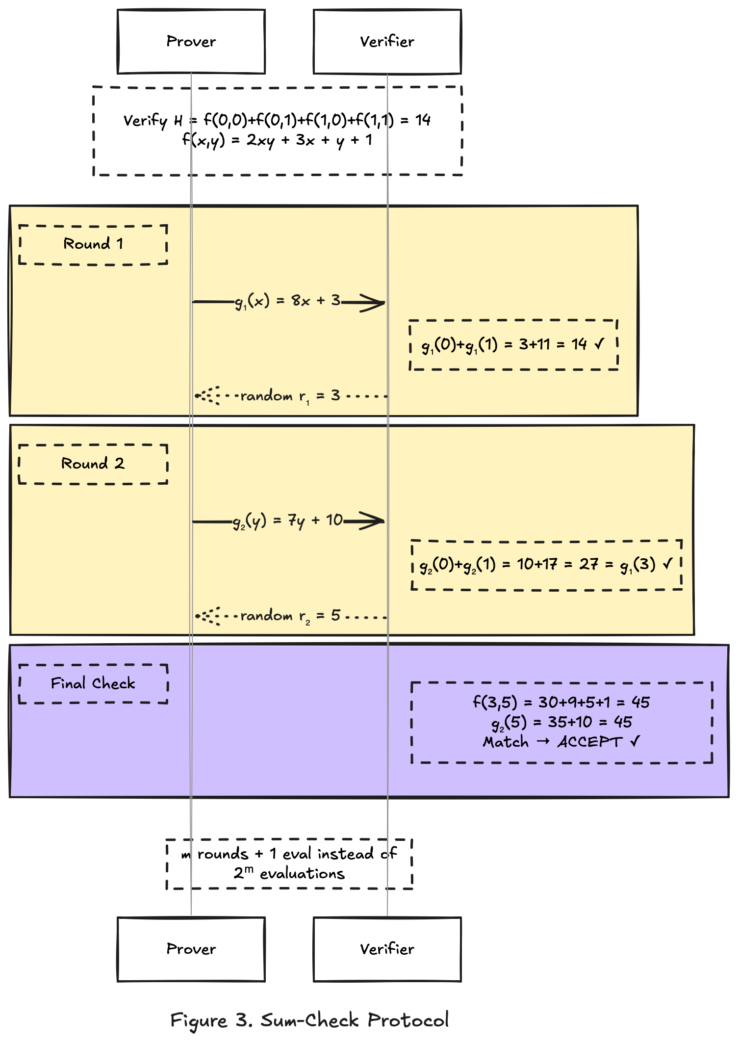
Let f(x, y) = 2xy + 3x + y + 1.
The true values are:
f(0,0) = 1, f(0,1) = 2, f(1,0) = 4, f(1,1) = 7
H = 1 + 2 + 4 + 7 = 14.
Round 1: eliminate y
The prover “sums out” y, producing a polynomial in x alone:
g₁(x) = f(x, 0) + f(x, 1)
Expanding:
f(x, 0) = 2x·0 + 3x + 0 + 1 = 3x + 1
f(x, 1) = 2x·1 + 3x + 1 + 1 = 5x + 2
So g₁(x) = (3x + 1) + (5x + 2) = 8x + 3.
Consistency check. If the prover is honest, then g₁(0) + g₁(1) must equal H, because:
g₁(0) = f(0,0) + f(0,1) = 3
g₁(1) = f(1,0) + f(1,1) = 11
3 + 11 = 14 = H
This check alone does not prove correctness. The prover could have sent a different polynomial that also satisfies g₁(0) + g₁(1) = 14.
For example, g₁(x) = 14x passes: g₁(0) + g₁(1) = 0 + 14 = 14, but it is the wrong polynomial.
Random challenge. The verifier picks a random r₁ = 3 and evaluates g₁(3) = 8·3 + 3 = 27. This value becomes the target for the next round.
Here is why this works: if the prover lied about g₁, then by Schwartz-Zippel, the false g₁ and the true g₁ almost certainly disagree at a random point. The random challenge locks in the prover’s claim at a specific value, making it difficult to maintain a consistent lie in later rounds.
Round 2: eliminate x (now fixed at r₁ = 3)
The prover computes:
g₂(y) = f(3, y) = 2·3·y + 3·3 + y + 1 = 7y + 10
Consistency check. The verifier checks that g₂(0) + g₂(1) equals the target from Round 1:
g₂(0) = f(3, 0) = 10
g₂(1) = f(3, 1) = 17
10 + 17 = 27 = g₁(3)
This links Round 2 back to Round 1. If either round contains a lie, this equation breaks with high probability.
The verifier picks r₂ = 5 and evaluates g₂(5) = 7·5 + 10 = 45.
Final check: verify against the original polynomial
All previous checks ensured internal consistency between rounds. But they were all based on polynomials sent by the prover. The verifier has not yet touched the original polynomial f.
Now the verifier computes f(r₁, r₂) = f(3, 5) directly:
f(3, 5) = 2·3·5 + 3·3 + 5 + 1 = 30 + 9 + 5 + 1 = 45
Compare: g₂(5) = 45 = f(3, 5)
This step ties the prover’s claims back to the actual polynomial. Without it, the prover could have constructed rounds that are internally consistent but have nothing to do with f.
Why the prover cannot cheat
Each round forces the prover to commit to a polynomial before seeing the random challenge. If any committed polynomial differs from the honest one, Schwartz-Zippel catches the discrepancy with probability at least 1 - d/p.
A lie in Round 1 propagates to Round 2 through the random challenge, and collides with the final direct evaluation.
Efficiency
The verifier performs m rounds of: receiving a low-degree polynomial, checking one equation, and sampling one random point. The final step is a single evaluation of f. Total work: O(m) instead of O(2^m).
For m = 30: about 30 operations instead of one billion.
Committing to polynomials: making claims binding
The Sum-Check protocol assumes the prover can “send” a polynomial to the verifier. In the walkthrough, the prover sent g₁(x) = 8x + 3. But what does “send” mean concretely?
If the prover sends the polynomial’s coefficients, the verifier receives them, and the protocol works. But for large polynomials, this is expensive. And more importantly, the prover could send one polynomial in Round 1 and quietly swap it in Round 2. The protocol needs a way to lock the prover into a specific polynomial cheaply.
A polynomial commitment scheme has three operations. The prover first computes a short fingerprint of the polynomial, called a commitment, which is a single group element regardless of the polynomial's size. Later, the verifier picks a random point r and asks for f(r). The prover responds with the value and an opening proof. The verifier checks the proof against the commitment. If the prover lied about f(r), verification fails.
The commitment is binding. Once sent, the prover cannot change the polynomial without being caught. The binding property turns the interactive Sum-Check protocol into something enforceable.
Jolt uses a commitment scheme based on multiscalar multiplication (MSM). The key property: when the committed values are small (say, entries from a lookup table that fit in a few bits), the MSM cost drops significantly compared to committing arbitrary field elements. This matters because Lasso’s lookup tables produce exactly this situation. The committed field elements are small even though the underlying finite field is large.
Other proof systems use different commitment schemes. KZG commitments require a trusted setup. FRI (used by STARKs) avoids trusted setup but produces larger proofs. Jolt’s MSM-based approach sits between them: no trusted setup, and prover cost scales well when committed values are small.
The rest of this article assumes polynomial commitments exist and work. The important point is that every time the prover “sends a polynomial,” it actually sends a commitment, and every evaluation is backed by an opening proof that the verifier checks.
Lookup argument: replacing computation with table lookup
The Sum-Check protocol verifies polynomial sums efficiently. Polynomial commitments make the prover’s claims binding. To prove CPU execution, one more idea is needed.
The problem with circuits
Suppose we want to prove that a CPU correctly executed an ADD instruction: ADD(3, 4) = 7.
The traditional approach encodes this as an arithmetic circuit:
a + b - c = 0The prover assigns a = 3, b = 4, c = 7, and proves the constraint is satisfied.
This works for ADD. But a CPU has dozens of instructions. Each one needs a different circuit: AND requires bitwise decomposition, SLT (set-less-than) requires comparison logic, MULHU (unsigned upper multiply) requires carry propagation. Each circuit must be hand-written and audited. Bugs in any single circuit break soundness.
The lookup alternative
Jolt takes a different approach. Instead of proving the computation directly, it proves that the input-output triple exists in a precomputed table.
For ADD: the prover shows that (3, 4, 7) appears in a table containing all valid additions.
For AND: the prover shows that (0b1010, 0b1100, 0b1000) appears in a table containing all valid bitwise ANDs.
The same protocol handles every instruction. The prover never constructs instruction-specific circuits. It only proves membership in the correct table.
Adding a new instruction to the VM means adding a new table. No new circuits, no new constraint logic, no new audit surface.
The size problem
This idea has an obvious flaw. For a 64-bit ADD instruction, each operand has 2⁶⁴ possible values. The full table has 2⁶⁴ × 2⁶⁴ = 2¹²⁸ rows. No one can store or commit to a table with 2¹²⁸ entries.
Prior lookup arguments (plookup, Halo2’s lookup) required the prover to commit to the entire table. This made large tables impractical and confined lookups to small, hand-picked tables.
Lasso: decomposing large tables into small ones
Lasso solves the size problem by exploiting table structure.
Consider 16-bit addition. The full table has 2³² rows. But 16-bit addition decomposes into two 8-bit additions with a carry:
ADD(a, b) where a = (a_hi, a_lo) and b = (b_hi, b_lo)Step 1: Compute a_lo + b_lo. This gives a partial sum and a carry bit.
Step 2: Compute a_hi + b_hi + carry.
Each of these sub-operations only requires a table with 2⁸ × 2⁸ = 2¹⁶ rows (for 8-bit operands). That is 65,536 entries. Entirely manageable.
More generally, a 64-bit addition decomposes into eight 8-bit additions. The total table size becomes 8 × 2¹⁶ = 524,288 entries instead of 2¹²⁸.
Why decomposition works: the structure property
Not every table can be decomposed this way. Lasso requires that the table is decomposable, which means:
A single lookup into a table T of size N can be answered by performing c lookups into subtables T₁, T₂, ..., Tₗ, each of size N^(1/c), and then combining the results with a known function.
The combination function depends on the instruction: carry propagation for addition, concatenation for bitwise AND, and a more involved recombination for shifts.
The critical insight from the Jolt paper: all RISC-V instructions have this decomposable structure. Addition, subtraction, bitwise operations, comparisons, shifts, multiplications. Every one of them can be broken into small subtable lookups that recombine correctly.
How Lasso proves a lookup
Suppose the prover claims it performed m lookups into a table T, and each lookup returned the correct value.
Lasso needs to prove two things: that each subtable lookup returned the right entry, and that the subtable results were combined correctly. For the first, the prover commits to the subtable entries it accessed (small values, so MSM-based commitment is cheap). The verifier uses Sum-Check to confirm these values match the known subtable contents. For the second, the combination function (carry propagation, concatenation, etc.) is also verified through Sum-Check.
Because the committed values are small (they come from 8-bit subtables), the prover’s commitment cost is dominated by O(m + n) group operations, where m is the number of lookups and n is the subtable size. This is far cheaper than prior lookup arguments that scaled with the full table size.
Concrete example
A program executes two instructions:
ADD(300, 200) = 500
ADD(250, 30) = 280
The prover decomposes each into subtable lookups:
For ADD(300, 200): Decompose 300 into (1, 44) and 200 into (0, 200) as two 8-bit chunks.
Low byte: 44 + 200 = 244, carry = 0.
High byte: 1 + 0 + 0 = 1.
Result: (1, 244) = 256 + 244 = 500.
The chunks recombine without carry, but the high byte is nonzero, showing that the subtable split is not trivial for numbers above 255.
For ADD(250, 30): Decompose 250 into (0, 250) and 30 into (0, 30).
Low byte: 250 + 30 = 280, which overflows a single byte. 280 mod 256 = 24, carry = 1.
High byte: 0 + 0 + 1 = 1.
Result: (1, 24) = 256 + 24 = 280.
Here the low byte overflows. The carry bit propagates from the low subtable to the high subtable, and the combination function must account for it.
The prover commits to all subtable access values and combination results. The verifier checks, via Sum-Check, that every subtable access is valid and every combination is correct.
At no point does anyone materialize the full 2¹²⁸-row table. The verifier evaluates the subtable polynomials directly at random challenge points, using the fact that the subtables are small and their multilinear extensions can be computed efficiently.
Jolt: proving a full CPU execution
Lasso proves that individual lookups are correct. A running CPU does more than individual instructions. It fetches instructions from memory, reads and writes registers, and follows a program counter that jumps and branches. Jolt combines Lasso with three other mechanisms to cover the full execution.
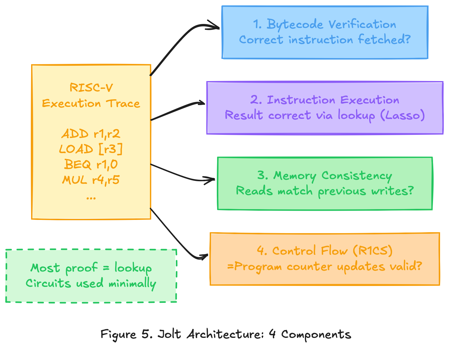
Component 1: Instruction execution (Lasso lookups)
This is the core. Every RISC-V instruction in the execution trace is proven correct via Lasso lookup, as described above.
The prover generates an execution trace: a step-by-step record of what the CPU did. For each step, the trace records the instruction, the input operands, and the output.
Component 2: Bytecode consistency (offline memory checking)
The CPU must fetch the correct instruction at each step. If the program has instruction “ADD r1, r2, r3” at address 0x04, then whenever the program counter equals 0x04, the fetched instruction must be ADD with those operands.
This is a memory consistency problem. The program bytecode is stored in memory. The CPU reads from it at every step. Jolt needs to ensure that every read returns the correct value.
Jolt uses offline memory checking, a technique from the Spice protocol (optimized with Lasso). The idea:
Think of memory as a sequence of (address, value, timestamp) tuples. Every read operation must return the value from the most recent write to that address. To verify this, the prover sorts all memory operations by address, then by timestamp. Adjacent operations on the same address must form valid read-after-write pairs. This constraint is expressible as a polynomial identity, checkable via Sum-Check.
For bytecode specifically: the program is written once (at “time 0”) and only read during execution. So the check simplifies to confirming that every instruction fetch matches the original bytecode at that address.
For example, address 0x04 is written at time 0 with value ADD. The CPU reads 0x04 at time 5 and again at time 12. The checker verifies both reads return ADD.
Component 3: Read-write memory (registers and RAM)
The same offline memory checking technique applies to registers and RAM, but now with both reads and writes during execution.
When the CPU executes “ADD r1, r2, r3”, it reads the values in registers r1 and r2, computes the sum, and writes the result to r3.
The memory checking argument ensures that values read from r1 and r2 match the most recent writes to those registers, and that the write to r3 is recorded correctly for future reads.
Lasso handles range checks within this component. When the memory checker needs to verify that a timestamp is in a valid range, it treats the range check as a lookup into the table [0, 1, ..., m-1]. This keeps everything within the lookup framework.
Component 4: Control flow (R1CS constraints)
The program counter must advance correctly. This is the one part of Jolt that uses traditional arithmetic constraints instead of lookups. For sequential instructions, PC increments by the instruction size. For branches, PC jumps to the target if the condition is true and increments otherwise.
These constraints are simple linear relations. They glue the execution trace together, ensuring that each step follows from the previous one according to the program’s control flow.
How the components connect
The four components share the same execution trace. Instruction execution proves each step is computed correctly. Bytecode consistency proves the right instruction was fetched. Memory consistency proves that register and RAM reads/writes are valid. Control flow proves the program counter advanced correctly.
Each component produces a separate set of polynomial claims. The verifier checks all of them using Sum-Check and polynomial commitment openings. If any component fails, the overall proof is rejected.
The architecture is deliberately lookup-heavy. Three of the four components rely on Lasso (instruction execution, bytecode, memory). Only control flow uses R1CS, and those constraints are simple. This uniformity is what makes Jolt simpler than prior zkVMs, where each component often required a different proving technique.
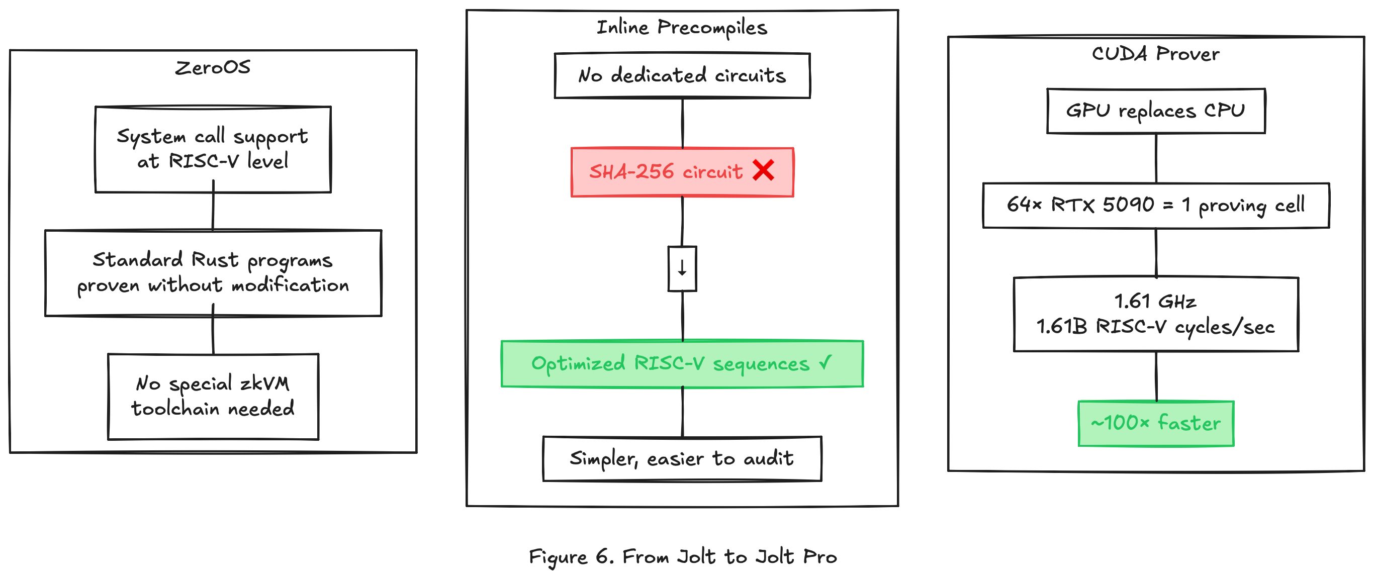
From Jolt to Jolt Pro
Jolt is an open-source zkVM from a16z. It runs on CPU and proves RISC-V execution using the lookup architecture described above.
Jolt Pro is LayerZero’s fork. It targets a specific operational requirement: prove blocks fast enough that validators can verify proofs in real time, within the block time of the Zero chain. This is not an academic benchmark target. If the prover cannot keep up with block production, the chain stalls.
Three modifications move Jolt toward this target.
1. GPU-accelerated prover
The most performance-critical operation in Jolt is the multiscalar multiplication (MSM) used in polynomial commitments. MSM computes a weighted sum of elliptic curve points:
C = a₁·G₁ + a₂·G₂ + ... + aₙ·GₙThis operation is embarrassingly parallel. Each scalar-point multiplication is independent, and partial sums can be combined in a tree structure. GPUs, with thousands of cores optimized for parallel arithmetic, are a natural fit.
Jolt Pro runs the prover on GPU clusters. A proving cell consists of 64 colocated NVIDIA RTX 5090 GPUs. On this hardware, the prover achieves 1.61 billion RISC-V cycles per second (1.61 GHz).
For context: Jolt on CPU proves in the low tens of millions of cycles per second. SP1 and RISC Zero, also CPU-based, operate in a similar range. The 100x speedup claim compares a 64-GPU cluster against single-machine CPU provers. It is a real performance number, but it reflects a hardware difference as much as an algorithmic one. A fairer comparison would normalize by cost (dollars per proven cycle), which LayerZero has not published.
The roadmap targets 4 GHz per cell by 2027, presumably through a combination of hardware upgrades and further MSM optimization.
2. Inlines instead of precompiles
Other zkVMs (RISC Zero, SP1) add “precompiles” for expensive operations like SHA-256, Keccak, or elliptic curve arithmetic. A precompile is a dedicated circuit, hand-optimized for that specific operation, that runs alongside the main VM proof.
Precompiles are fast for the operations they cover. But each one is a separate constraint system that must be independently designed, implemented, and audited. A soundness bug in a single precompile breaks the entire proof. As more precompiles are added, the audit surface grows.
Jolt Pro takes the opposite approach. Instead of precompiles, it uses “inlines”: optimized sequences of standard RISC-V instructions that implement the same operation. SHA-256 is expressed as a series of ADD, XOR, SHIFT, and AND instructions. Each of those instructions is proven through the same Lasso lookup pipeline as everything else.
Inlines are slower to prove per operation than a hand-tuned precompile would be. But they eliminate the need for operation-specific circuits entirely. The entire prover runs through one uniform code path, compensating for per-operation overhead with raw GPU throughput and gaining auditability in return.
Whether this tradeoff holds depends on workload composition. If a program spends 90% of its cycles on SHA-256, a precompile-based system will be more efficient. If the workload is diverse (general smart contract execution), inlines suffer less of a penalty and the simplicity advantage dominates. Zero targets EVM execution for financial applications, which tends to be diverse.
3. ZeroOS: system call support
Vanilla Jolt proves pure computation: a function takes inputs and produces outputs, with no interaction with the outside world. A running program needs more than that. It needs to allocate memory, read input data, write output data, and access environmental information (block number, timestamp, caller address).
ZeroOS adds a system call layer at the RISC-V level. When the guest program executes an ECALL instruction (the RISC-V system call mechanism), ZeroOS intercepts it and handles the request. The prover includes the system call inputs and outputs in the execution trace, and Jolt’s memory checking ensures consistency.
This means standard Rust programs, compiled to RISC-V with a thin runtime, can be proven without modification. The developer writes normal Rust, uses standard library features (allocation, I/O, formatting), and the compiled binary runs inside the Jolt Pro prover as-is.
Without ZeroOS, guest programs would be limited to pure functions with fixed-size inputs, the way most current zkVM guest programs are written. ZeroOS removes that constraint, which is necessary for running a full EVM implementation inside the prover.
What Jolt Pro does not change
Jolt Pro does not modify the underlying cryptographic protocol. The Sum-Check arguments, Lasso lookup decompositions, offline memory checking, and R1CS constraints are the same as in Jolt. The polynomial commitment scheme is the same MSM-based approach. The soundness guarantees are inherited from the original Jolt construction.
The modifications are at the engineering layer: where the computation runs (GPU vs. CPU), how complex operations are expressed (inlines vs. precompiles), and what the guest program can do (system calls vs. pure functions). The math underneath is unchanged.
Open question: auditability
Jolt is open source under a16z. Jolt Pro is not. The proof is publicly verifiable: anyone can check a Jolt Pro proof against the verification algorithm. But the prover implementation — the code that generates proofs — cannot be independently reviewed.
This matters for two reasons. First, a bug in the prover could generate invalid proofs that happen to pass verification (a soundness failure). Second, institutions evaluating Zero for financial infrastructure will want to audit the full stack, not just the verifier. The closed-source prover creates an asymmetry: the math is trustless, but the implementation requires trusting LayerZero.
Whether this is acceptable depends on the threat model. If verification is sound, a buggy prover only hurts the prover (it might fail to generate valid proofs, not generate false ones). But proving this argument rigorously requires seeing the code.
Open questions
Several points remain unresolved.
Performance claims are based on demo environments, not mainnet workloads.
Hardware costs are high. A single proving cell requires 64 GPUs.
Only a small number of entities may produce blocks, raising censorship concerns.
What comes next
This article covered the path from polynomial arithmetic to Jolt Pro.
Jolt Pro is one part of the Zero stack. Other components include:
QMDB: ZK-optimized state database
FAFO: parallel execution scheduler
SVID: data availability scheme
Future articles will cover these.
The goal is to allow validators to verify proofs instead of re-executing transactions. This enables parallel execution across independent environments, called Atomicity Zones.
Each zone functions like a full EVM, but runs in parallel. This removes the single-thread bottleneck found in most blockchains.
Zero’s Atomicity Zones are governed by a single protocol. Ethereum’s rollups are independently operated, each with its own security assumptions and upgrade governance. This difference matters for financial institutions: a single protocol means one audit target, one trust boundary, and one set of security guarantees.
For infrastructure targeting financial institutions, this distinction determines system design, security guarantees, and trade-offs.
The math is the same. The design choices differ.
This is Article 1 of the Dissecting Zero series.
Next: QMDB and ZK-native state storage.
I am a blockchain platform engineer at B-Harvest. Over the past two years, I have operated validator and RPC infrastructure across more than ten networks and contributed to core chain development with Cosmos SDK and CometBFT. My current focus is building a development tooling platform for financial institutions entering Web3.
Feedback is welcome. Reach out on LinkedIn or Twitter (@jinuahn05).